
Monte Carlo option pricer on an FPGA
A fully pipelined fixed-point option pricer that simulates one price path every clock cycle.
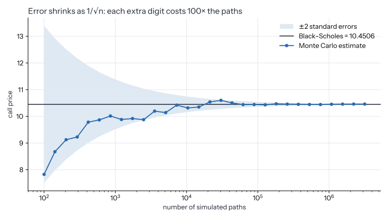
A Monte Carlo pricer estimates an option's value by simulating many random price paths and averaging their payoffs. The catch is the error: it shrinks only as 1/√n, so every extra digit of accuracy costs 100× more paths. I built a pricer in hardware to make paths cheap: fully pipelined, in fixed point, finishing one path every clock cycle on a Lattice ECP5-85F.
The pipeline
The design is built from xorshift random number generators, a CLT Gaussian adder tree and a block-RAM exponential unit. Each stage passes a valid bit to the next: z, x, e (three cycles through the exp unit), s and p, into the running sum. The RTL's prices land within 2σ of Black-Scholes.
The letters are the signal each stage produces, named after the math:
- z: the standard normal sample Z ~ N(0,1), the sum of 12 uniforms minus 6.
- x: the exponent x = a + b·Z, where a = (r − σ²/2)T and b = σ√T. This is the stock's log-return over the year.
- e: eˣ, the growth factor for the path. It takes 3 cycles: the table read plus two pipeline registers.
- s: S_T = S₀·eˣ, the simulated stock price at expiry.
- p: the payoff, max(S_T − K, 0): what the call option pays on this path.
Sizing the numbers
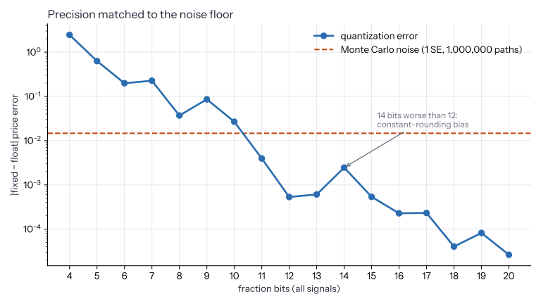
I sized the datapath with a fixed-point error sweep across every fraction width from 4 to 20 bits. Rounding error came out 28× below the Monte Carlo noise. The sweep also uncovered a systematic rounding bias that grew as fractional bits were added: 14 bits did worse than 12.
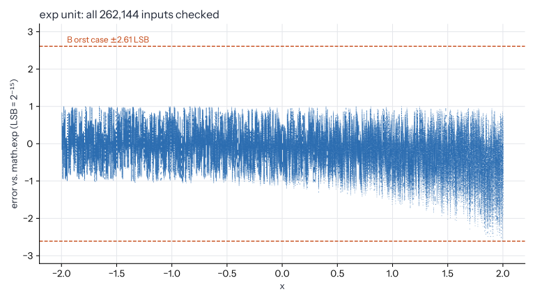
The exponential unit was checked against math.exp on all 262,144 inputs. The worst case is ±2.61 LSB, with one LSB = 2⁻¹⁵.
Making it fast
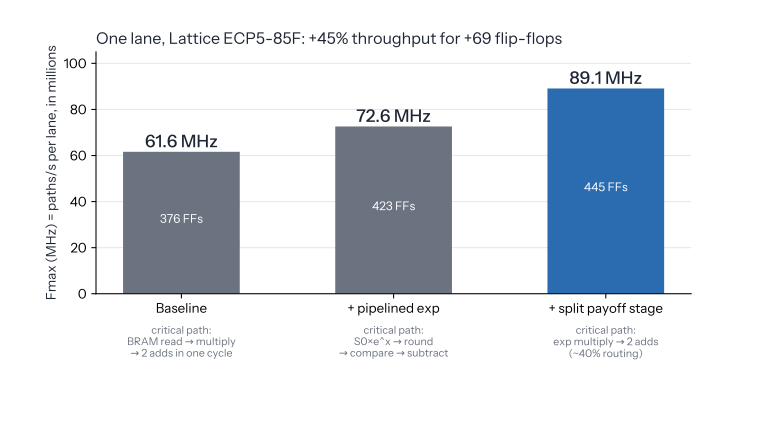
Two rounds of critical-path pipelining raised Fmax from 61.6 to 89.1 MHz, a 45% gain, for 69 extra flip-flops. Pipelining the exp unit reached 72.6 MHz; splitting the payoff stage reached 89.1 MHz. The remaining critical path is the exp multiply into two adds, with about 40% of its delay in routing. At one path per cycle, Fmax is throughput: 89.1 million paths per second from one lane.
- after an 8-cycle pipeline fill
- 1 path / cycle
- Fmax, up from 61.6 (+45%)
- 89.1 MHz
- flip-flops for the speedup (376 → 445)
- +69
- rounding error below Monte Carlo noise
- 28×
Proving it right
Every block is verified bit-exact against Python models in cocotb: 9 tests, about 6,000 random vectors and 13 corner cases. On top of that, the exp unit was checked exhaustively, on all 262,144 inputs.